20.1 Google Sheets 🎯
This section includes an Activity 🎯
In your product management career, you'll use many different tools to analyze data and understand how your product is doing. Spreadsheet applications like Microsoft Excel or Google Sheets are a popular tool for this kind of analysis. Spreadsheet apps accept a wide variety of data, are easy to manipulate, and provide lots of built-in functions. In addition, many of them include data visualization features that can turn data insights into impressive, easy-to-understand visuals. Analyzing and presenting data is a crucial PM skill.
In this checkpoint, you'll learn and practice a few data analysis skills using Google Sheets. The checkpoint focuses on Sheets because Google Suite, which Sheets is included in, is extremely popular with tech companies and is free to access (you just need a Google account). However, the principles you will learn here are highly transferable to other spreadsheet apps.
If you're new to using spreadsheets, this will be a core skill to develop in preparation for product roles. If you're an intermediate spreadsheet user, this checkpoint will be an opportunity to refresh and expand your skills. And if you're already a spreadsheet master, you might still learn a few tips and tricks that you didn't know. You should also use this opportunity to consider how spreadsheets can be used in product management work.
By the end of this checkpoint, you should be able to do the following:
- Effectively use Google Sheets to perform product-related data analysis

Getting started with spreadsheets
This checkpoint focuses on applying spreadsheet functions to product work and assumes you have already mastered basic spreadsheet skills like selecting cells, creating simple functions, etc. In fact, at this point you've already completed an assignment with Google Sheets in an earlier checkpoint about visualizing data. If you're new to Sheets—or to spreadsheets in general—it is highly recommended that you spend some time now refreshing your memory or learning the basics. Google maintains comprehensive support documentation for Sheets, and there are plenty of other resources online, like this spreadsheet guide from Zapier and various video tutorials on YouTube.
Formatting and sorting cells
When doing product data analysis in Sheets, the first thing you might want to do is tweak the text and format the data. This will make your spreadsheets more usable and understandable. For example, say you imported a CSV file with the following business data:
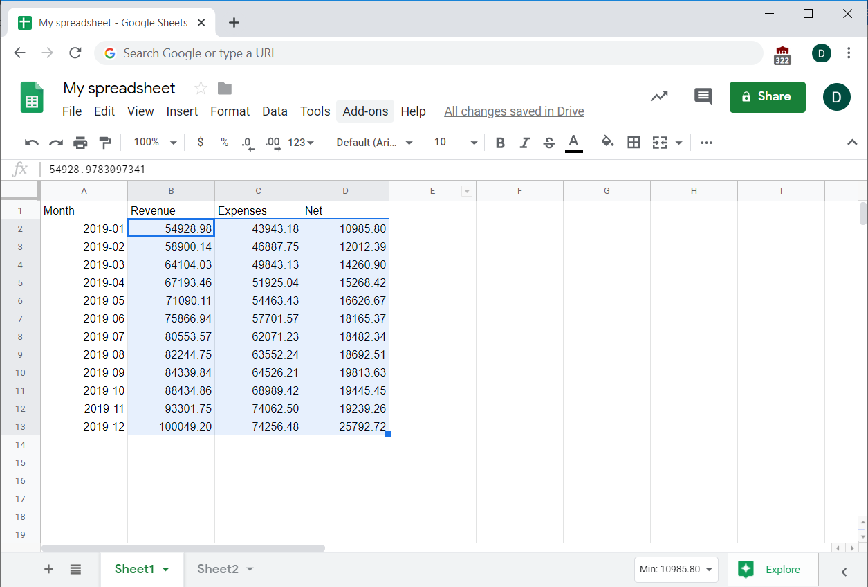
It looks a bit weird, right? That's because the data was imported as plain numbers instead of dollar figures. How can you change that? First, select the columns with the numbers you want to format. Then, under the Format menu, select Number, and then the Currency option. Your numbers will turn into dollar figures, making the information in the spreadsheet clearer:
Another handy use of formatting tools is to make your headers more visually distinct. To do this, select the row with the labels, choose the Bold option in the toolbar, and then choose Center for the text alignment. Suddenly, it looks much more like a table:

Finally, you might want to sort the data, especially if it wasn't sorted in the first place. Say you want to see the data sorted by Expenses. First, select the data you want to sort—in this case, you'll select the whole sheet. Then choose the Data menu and select the Sort Range option. Check the Data has header row box (this excludes your header from being sorted), then choose the Expenses column. Poof, your data is sorted from the smallest expense to the largest one:
Basic math formulas
On the most basic level, you can use spreadsheets to make simple math calculations quick and easy. For example, imagine that the net column information (representing the net profit for each month) was missing from your original file, and you only had the data for the revenue and expenses. You could easily calculate the net value, which equals revenue minus expenses. In the below spreadsheet, you would do this by selecting an empty cell (here, F8 is selected) and entering a formula to calculate the net value: =B8-C8.
Since you do have that information, you can compare the result to the one in cell D8, and verify that the formula properly calculated the net value. Next, you can easily expand this formula to calculate the net value for every row in the sheet. To do this, place your cursor on the square at the bottom right of the selected cell containing the formula, and drag to apply the formula to a range of desired empty cells. Alternatively, you can just copy the formula, select the cells you want to paste it into, then hit Paste. This works with either the Edit menu or your keyboard shortcuts:
As you'll note in the screencast above, this does not result in the formula from F8—which you'll recall was =B8-C8—being copied "as is" to the new cells. If it did, every cell in column F would have displayed the same number: $18,482. Instead, each new cell in column F is calculating the revenue and expenses information relevant to its own row. The formula for F7 is =B7-C7, and for F6 it is =B6-C6, etc.
This happens because Sheets (and most spreadsheet tools) uses the cell's position to make the formula work in its new destination cells. The formula you pasted from F8 was automatically changed to reflect the relative positions of each of the new cells involved.
Another simple math formula you're likely to use often is summation. The formula for returning a sum is =SUM([range]), where [range] is either a cell or a range of cells that will be summed together. If you apply this formula to an individual cell, for example by writing =SUM(C8), it will return the exact same value as =C8. If you want to sum a range of numbers, you can specify a range by listing its first and last cells with a colon (:) in the middle.
For example, suppose you wanted to add a total revenue column to the sample spreadsheet you've been using. One way to do this is to just add up the individual cells, like =B2+B3+B4+…, but that gets tedious quickly and might be impossible with larger datasets.
Choose an empty cell (such as B15), enter the SUM formula, and specify the range. In this case, the range would be between B2 and B13, written like this: B2:B13. And the formula is =SUM(B2:B13).
Ranges can span both rows and columns. If you need to manipulate the entire range of numbers in the sheet in one formula, the range to specify would be B2:D13.
Note in the screencast above that when you type in a formula, Sheets will give you suggestions for formulas and details on how the formula you typed in works. This is a great example of product onboarding; including this feature in Sheets provides users with a handy reference point in case they forget the details of a complex formula or need to verify what it does.
Simple math formulas (addition, division, subtraction, and multiplication) can also be used with plain numbers instead of cell addresses. For example, say your sales team gets a 10% commission on revenue. You could easily calculate the sums of their commission by using a formula to multiply every value in the Revenue column by 10%:
COUNT and COUNTIF
Imagine you work for an online video rental service. Your sales team has a new potential film distributor, but they need a few questions answered to seal the deal. You don't have access to the database, so your engineers did a quick database dump into a few CSV files that you imported into Sheets.
First, the sales team wants to know how many G-rated films you have. The formula for counting items is =COUNT(range). Remember that most spreadsheets have header rows; you should exclude the headers from your count. Looking at the grid, you can see that the data begins on row 2 and ends at row 1001, so =COUNT(D2:D1001) gives 1000 films:

Note that this formula counted only one column. If you count across two columns—say by using =COUNT(C2:D1001)—you'll get 2000 items, which is not the right answer!
Now, how many of those 1000 films are rated G? To figure this out, you'll need a new function: COUNTIF. This function takes two parameters. The first is the range that you want to match. The second is the condition that you want to match. If the condition matches what's in the cell, it gets counted. If it doesn't match, it doesn't get counted. So, if you want to count only G-rated movies, you'd count over column E like so: =COUNTIF(E2:E1001, "G").
And just like that, you'd get the answer: 178 movies. You can check your work by counting all the movies that aren't rated G. The "condition" in COUNTIF will let you test for items greater than (>), less than (<), and not equal to (<>) that value. So, if you want to find all the movies that are not rated G, you'd use the "not equal to" condition like so: =COUNTIF(E2:E1001,”<>G”). Then let Sheets take care of the rest. It comes out to 822 movies!
Check your results: 822+178=1000 movies. You can be confident that the answer you reached on the number of G-rated movies is correct, and return to your sales team with a correct answer.
Averages and medians
The next question your sales team asks you is what's the average payment price of a rented film. For this one, you'll use the AVERAGE function. This function averages the items in the range you give it. In this case, it's =AVERAGE(E2:E16050).
The function returned a number of $4.20. Note that the dollar formatting didn't get applied to the average field. You'll want to take a minute to format it so that it's easily understood.
It's also worthwhile to look at the median value—that is, the "middle" value of all the numbers. Why? Well, if the median is far off from the average, it's a sign that there are some really big or really small numbers (known as outliers) that could be inflating or deflating the average. For example, imagine that you have 100 rentals, 99 of which are $1 and one of which is $1000. The median value is $1, but the average value is $10.99. One single $1000 rental makes your average very misleading! For this reason, it is always best practice to examine the median alongside the average. You can use the MEDIAN function to find the value:
In this case, the median is $3.99, which is close to the $4.20 average. This indicates that the average is reliable; there are probably no big or small outliers that skew the average.
Advanced functions
Spreadsheet apps like Sheets can do more sophisticated data analysis. The functions in this section are more difficult, but provide an invaluable tool for the day-to-day work of product managers. Keep reading to level up your Sheets data analysis skills!
UNIQUE and cross-sheet references
Say that you want to investigate the habits of your online video rental customers. Specifically, you are interested in how many movies different customers rent. Your dev team couldn't give you the data from the customer database because it includes sensitive information, like credit card numbers, and was impossible to clean, or remove the sensitive information. But you're a savvy spreadsheet master, and you have another source of data that provides you with the rental information, which includes a customer ID for each rented film. How can you use this Sheet of rental information to create a list of customers by ID without any duplications?
The UNIQUE(range) function takes what's in a range of data and removes any duplicates, returning a list of just the unique items. You want to create the customer list without compromising the rental data, so you duplicate the information into a new sheet and label it Customer. Next, you'll need to connect the data in your new sheet to the original source, since the information isn't housed all in one sheet. How do you make a function refer to data in another sheet? There are two ways to do this.
One option is to select the cells you want in the formula. After you type the opening parenthesis in the formula, switch to the tab where you want the data to come from and select it. Close the parenthesis and hit enter, then your data will appear. Note that the exclamation point you see in the screencast below acts as a separator between the sheet you are referencing (in this case Rental) and the cell you are pulling from (in this case D2):
The second option is to type in the range. For a range within a sheet, recall that you type the first cell number, a colon (:), then the last cell number. But how do you indicate that a range is in a different sheet? You first write the name of that sheet, Rental, then an exclamation point (!), and then the range you want to use in that sheet, so =UNIQUE(Rental!D2:D16045).
As you can see, by using the UNIQUE(range) function, you were able to get a consolidated list of all of your customers' ID numbers without any duplicates.
Absolute addresses
Now you can count up the number of rentals for each customer. Remember the COUNTIF function? It works across sheets too. Your next move is to count the number of times each customer ID appears in the rental table. First, you figure out the formula for the first one. Here you're counting the number of times that the ID appears, so you're going to count over the D column in the Rental sheet—that is, Rental!D2:D16045. But what are the criteria? You want the function to count an item only if it matches the customer ID in the CustomerID column, so A2, A3, A4, etc.
For the first customer ID in columnn A, row 2, the formula is =COUNTIF(Rental!D2:D16045, A2). For the next row, it's =COUNTIF(Rental!D2:D16045, A3). What's the difference between these formulas?
Note that the only thing that changed between these formulas is switching from A2 to A3. You're still counting over the same D2:D16045 range. You might be tempted to enter that first formula and copy and paste it into the remaining fields. Look at what happens if you do that:
When the formula was pasted, the numbers changed. It's no longer D2:D16045, but rather D3:D16046. That's not what you want! This happens because cells will try to update their formulas according to their new location whenever you copy and paste a formula. If you copy it down one row, the spreadsheet thinks that you want to do the same formula on the next row, so SUM(A2:C2) copied down one row will become SUM(A3:C3). That's often exactly what you want, but not in this case. How can you stop this automatic adjustment?
To make a spreadsheet avoid adjusting the formula when you copy and paste it into a new field, you need to put a $ before the row and/or column that you want to freeze. So if your formula includes A$2, you are telling Sheets that if this is copied it's okay to update column A to whatever the new column is, but that row 2 must stay row 2. If you want to freeze just the column, put the $ before the column: $A2. And if you want to freeze both, put the $ character before both the column and the row, like this: $A$2. The $ sign in a formula tells Sheets that these are absolute addresses—ones that won't change when copied or moved.
Now you know everything you need to know to update the formula. You don't want the range D2:D16045 to change as you copy this formula, but you do want the condition to update, as it should always match the row you're in. So the new formula is: =UNIQUE(Rental!$D$2:$D$16045, A2).
And now you can copy and paste this into the spreadsheet for all of the customers.
When you are done, the result will look something like this:
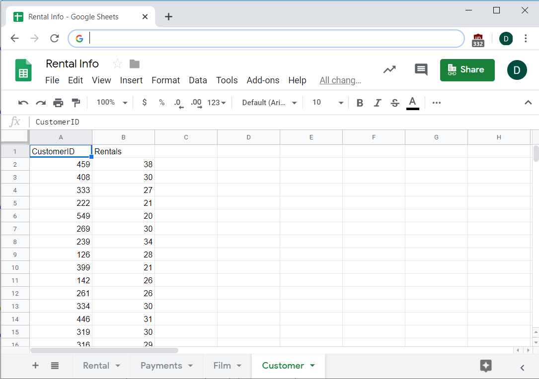
Now you have a list of every customer and their rental count, and you can be confident that it's accurate thanks to what you learned about absolute addresses. You can use absolute addresses in any formula, not just the one above.
VLOOKUP
There’s one last function you should learn: VLOOKUP. You should recall that in SQL you learned about using the JOIN function to merge two datasets. Similarly, VLOOKUP lets you merge sheets by matching a value in another sheet and returning data from that sheet.
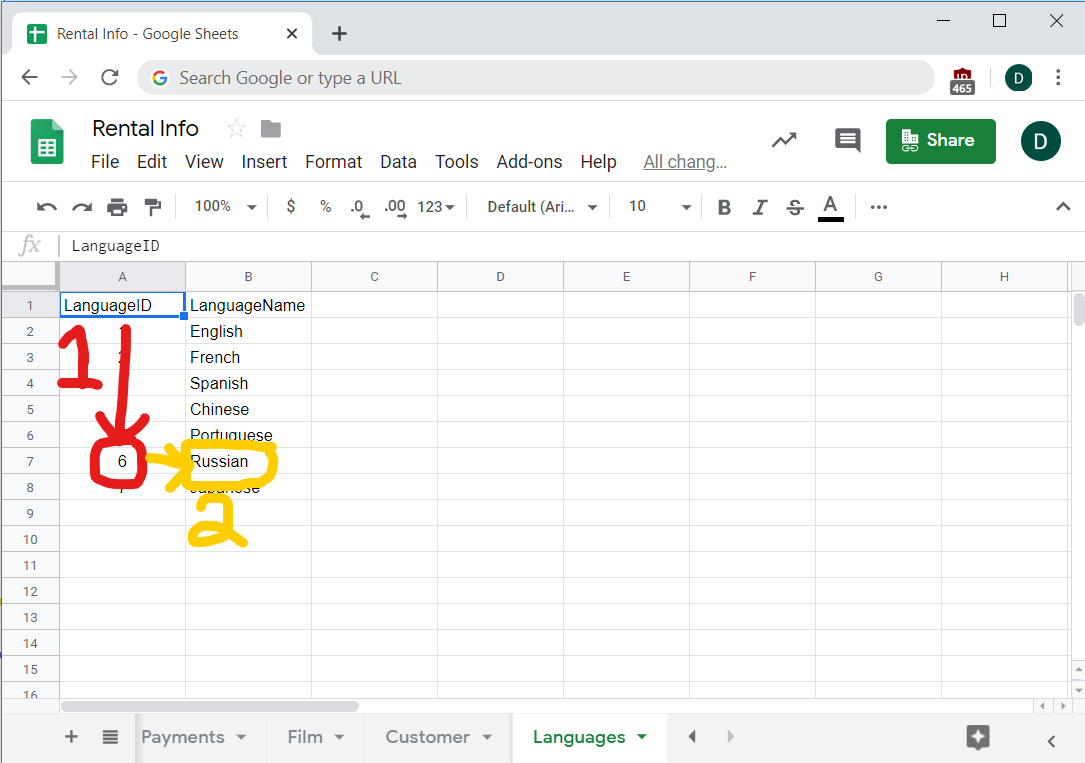
For example, check the Film sheet and LanguageID column. It would be really nice if instead of numbers you just had the language name. How can you combine the Language and Film sheets so that each film has the name of the language in it?
A VLOOKUP (or value look up) formula will take a value, like LanguageID, look for it in another range, then return a column from that range. For example, the first film has a Language ID of six. A VLOOKUP in the Language sheet would first go down the LanguageID column until it finds a match for six, then go to the column you designated—the second one in our case—and return the value there, which is Russian.
The VLOOKUP formula encapsulates all this. Here's how to break it down:
=VLOOKUP(search_key, range, index, [is_sorted])
The search key is the value you want to search for—in this case, it's the Language ID in the Film table. You'll put this in the Film sheet, so for the second row, the formula begins:
=VLOOKUP(F2…
The range is the range of values that includes both the item you're matching and the item that you want returned. In this case, this is all the data in the Languages table, not including the header row. You'll also make these absolute references. You'll want to copy and paste this formula, and it will not work properly if you forget the $ signs:
=VLOOKUP(F2, Languages!$A$2:$B$8…
The next parameter tells VLOOKUP which column in the range should be returned when it finds a match. The columns start with column A, so you want the language name to appear in column B:
=VLOOKUP(F2, Languages!$A$2:$B$8, 2…
The is_sorted value is optional, but really important. If you enter true or leave it blank, VLOOKUP will assume that all the values in the range are sorted. That means that if is_sorted is true and you're looking for six in this data, VLOOKUP will not find it because it's expecting the data to be sorted.

So, if your data isn't sorted, make sure to set is_sorted to false. Thankfully, the data in our case is in fact sorted, so you're done!
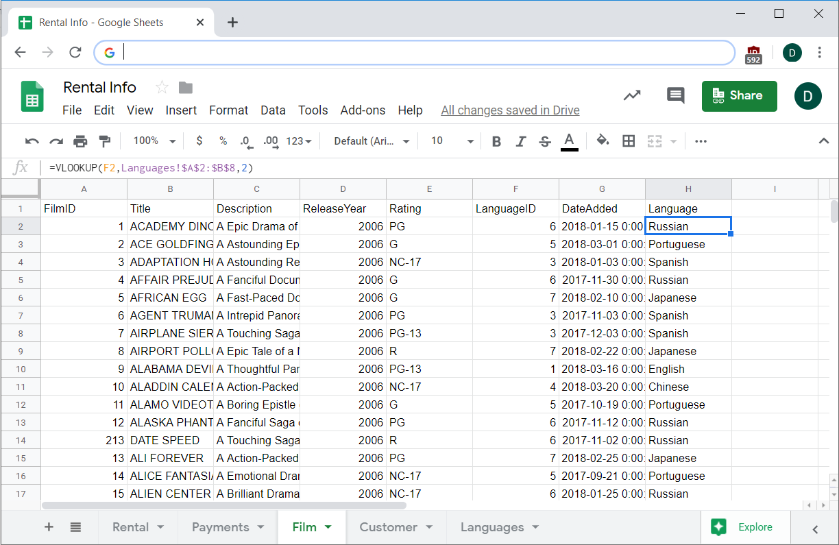
=VLOOKUP(F2, Languages!$A$2:$B$8, 2)
And it looks like this when you enter it:
Now you can copy and paste that formula in the whole column to see all the languages beside their films:
VLOOKUP is a very powerful function. It lets you visualize and merge data rapidly. It's useful when you need to simplify and clean up data so that you can make better sense of it, and it's also helpful when you just want to make the data more presentable and easily understood by a stakeholder. Take the time to practice VLOOKUP now. It's a tool you'll be glad to have in your arsenal when digging into data and presenting that data.
Activity 🎯
You are the product manager on an e-commerce platform. Here's a sample spreadsheet of some recent orders off your platform. This is the same data you were querying with SQL a few lessons ago. Now you can use your spreadsheet skills to calculate the following:
- Average number of items per order from the purchase_items sheet. Hint: Use the quantity column.
- Percentage of people who ordered multiple times. Hint: Use the quantity column on the purchase_items sheet to see what percentage of orders have a quantity that's greater than 1.
- Most popular item. Hint: There are 20 products, each with a unique ID of 1-20. Check to see which of these shows up the most in the product_id column of the purchase_items sheet.
- The top 10 customers by total number of purchases. Hint: Check to see which user ID shows up the most often in the user_id column of the purchases sheet.
Ask the community in the slack channels about the answers they got